
Abstract
This study examines the relationships between monetary policy, inflation, real economic activity, unemployment, and market volatility and the returns on US equities, 10-year Treasury bonds, and S&P 500 option-implied volatility, while investigating how these relationships vary across economic regimes. Using 360 monthly observations from January 1994 to December 2023, obtained from the Federal Reserve Economic Data (FRED), the Shiller S&P 500 dataset, and the Chicago Board Options Exchange (Cboe), the study employs unit-root tests, regression models with heteroskedasticity- and autocorrelation-consistent standard errors, vector autoregression (VAR), Granger-causality tests, impulse response analysis, Johansen cointegration tests, regime-interaction models, and a two-state Markov-switching regression. The findings reveal that higher inflation is significantly associated with lower Treasury bond returns, with a one-percentage-point monthly increase in year-on-year inflation corresponding to a 0.78% decline in bond returns. Lagged inflation changes also Granger-cause bond returns, while increases in policy rates exhibit a negative but less robust association with bond performance. Equity returns are primarily influenced by contemporaneous changes in the VIX, whereas macroeconomic variables explain approximately 5% of monthly equity-return variation and contribute little to explaining option-implied volatility. Furthermore, policy-rate increases are negatively associated with equity returns during calm market conditions and, to a lesser extent, before the 2008 financial crisis. The results demonstrate significant variations in equity-market sensitivities across recessionary, high-volatility, and high-inflation regimes, with stock–bond correlations shifting from negative toward zero when inflation exceeds 3%. By jointly examining equity, government bond, and options markets over three decades encompassing major economic disruptions, this study contributes to understanding regime-dependent financial market dynamics and provides implications for investors, portfolio managers, and policymakers. However, the monthly frequency of observations and recursive identification strategy limit causal interpretation, while the exclusion of swap markets and international financial markets offers opportunities for future research.
Keywords
Introduction
How macroeconomic conditions are transmitted to asset prices is a central question for both asset pricing and monetary economics. Arbitrage pricing theory (Ross, 1976) and the intertemporal capital asset pricing model (Merton, 1973) imply that state variables which alter expected cash flows or discount rates should be priced, and the empirical work that followed confirmed that industrial production, inflation and interest-rate spreads carry information about stock returns (Chen et al., 1986; Fama & French, 1989). Since then the literature has divided into several strands. High-frequency studies identify the reaction of stocks and bonds to monetary policy surprises (Bernanke & Kuttner, 2005; Gertler & Karadi, 2015; Rigobon & Sack, 2004), term-structure studies link yields to inflation and output (Ang & Piazzesi, 2003), and a separate body of work studies option-implied volatility and uncertainty (Bekaert & Hoerova, 2014; Bloom, 2009).
These strands are rarely brought together. Equity, bond and derivatives markets are usually studied in isolation, with different samples, variable definitions and methods, so it is difficult to compare how the same macroeconomic shock is reflected across instruments. In addition, much of the monthly evidence was estimated before the COVID-19 shock and the 2021–2023 inflation episode, a period in which the stock–bond correlation and the behaviour of volatility changed markedly (Baker et al., 2020; Campbell et al., 2017). Finally, regime dependence is often asserted rather than tested: evidence that sensitivities differ between recessions and expansions, or between high- and low-inflation environments, is frequently based on informal comparisons of sub-samples.
This paper addresses these gaps with a single, fully documented monthly dataset for the United States covering January 1994 to December 2023. We ask four research questions.
RQ1: How are changes in the federal funds rate and in inflation related to equity and Treasury bond returns?
RQ2: Is real activity, measured by GDP growth and unemployment, related to asset returns contemporaneously or with a lag?
RQ3: How is option-implied volatility, the price of S&P 500 index options expressed as the VIX, related to macroeconomic conditions and to asset returns?
RQ4: Do these relationships differ across economic regimes?
The study contributes to the literature in three ways. First, it estimates the same set of macroeconomic drivers against three instruments (equities, government bonds and index options) using identical data transformations, which allows a direct comparison of sensitivities across markets. Second, it tests regime dependence formally, using interaction terms with Wald tests, Fisher tests of correlation differences and a Markov-switching model, instead of relying on descriptive sub-period comparisons. Third, it distinguishes carefully between contemporaneous association, predictability (Granger causality) and causality, and it reports the full set of specification choices and diagnostics, so that every result can be replicated from public data.
The remainder of the paper is organised as follows. Section 2 reviews the literature and develops the hypotheses. Section 3 describes the data and methods. Section 4 reports the results, Section 5 discusses them, Section 6 sets out implications for stakeholders, and Section 7 concludes with limitations and directions for future research.
Literature Review and Hypothesis Development
Theoretical framework
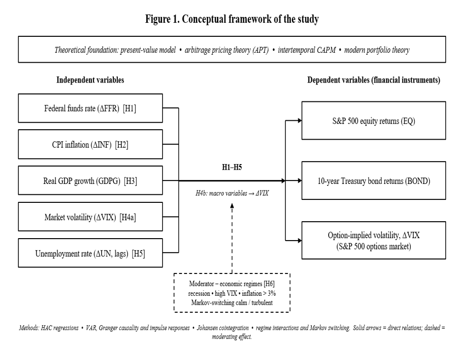
Our framework rests on three linked ideas. In the present-value model an asset price equals discounted expected cash flows, so any variable that changes expected dividends, the risk-free rate or the risk premium moves prices (Campbell & Shiller, 1988). Multi-factor models such as the APT and the ICAPM formalise this by treating macroeconomic innovations as systematic risk factors that command compensation (Merton, 1973; Ross, 1976; Chen et al., 1986), and the Fama and French (1993) model shows that common factors price both stocks and bonds. Portfolio theory (Markowitz, 1952), finally, implies that what matters for investors is not only each asset’s sensitivity but also how assets co-move, which is why cross-asset correlations and their regime dependence matter for allocation (Campbell & Viceira, 2002). Figure 1 maps the macroeconomic drivers to the three instruments and to the hypotheses developed below.
Monetary policy and asset prices
A higher policy rate raises discount rates and borrowing costs and should lower both stock and bond prices. Event studies find that an unexpected 25-basis-point cut in the federal funds rate raises broad stock indices by roughly one per cent, mainly through lower expected excess returns (Bernanke & Kuttner, 2005), and identification through heteroskedasticity confirms a negative effect of rate increases on equities (Rigobon & Sack, 2004). Earlier monthly VAR evidence points in the same direction (Thorbecke, 1997). More recent work shows that the equity response depends on what the announcement reveals: when a tightening signals stronger fundamentals, the “information effect” can offset the discount-rate effect (Jarociński & Karadi, 2020; Nakamura & Steinsson, 2018), and much of the apparent information effect reflects the Fed responding to public news (Bauer & Swanson, 2023). After 2008, forward guidance and asset purchases rather than the federal funds rate carried much of the policy stance (Swanson, 2021). Monthly studies that use the level or change of the federal funds rate report mixed results; Rincon and Vukovic (2024) find a negative valuation effect using instrumental variables, while Seip and Zhang (2022) show that lead–lag relations between GDP, Treasury yields and the federal funds rate alternate over time. The critical point from this literature is that monthly changes in the policy rate are endogenous to market conditions, because the Fed eases when markets fall, so a negative sign should be expected mainly in periods when policy is not reacting to financial stress. We state:
H1: Increases in the federal funds rate are associated with lower equity returns and lower Treasury bond returns.
Inflation, real activity and asset returns
Nominal bonds lose value when inflation rises because fixed coupons buy less and investors demand higher yields. The evidence that inflation news lowers bond returns is consistent across methods (Ang & Piazzesi, 2003; Campbell & Ammer, 1993; Flannery & Protopapadakis, 2002). For equities the picture is less clear. Fama and Schwert (1977) documented a negative relation between stock returns and inflation, which Modigliani and Cohn (1979) attributed to inflation illusion, but the sign has varied over time: Boons et al. (2020) show that the inflation beta of stocks changed sign around the early 2000s, and Campbell et al. (2017) link this to the switch of nominal bonds from “inflation bets” to “deflation hedges”. Real activity should raise expected cash flows and therefore equity prices (Chen et al., 1986; Fama & French, 1989), although the equity market also leads output, so contemporaneous links can be weak. Asymmetric and time-varying responses to macroeconomic variables are also reported for the US and Canada (Bhuiyan & Chowdhury, 2020) and for emerging markets such as India (Keswani et al., 2024), which suggests that single-regime linear estimates may hide offsetting effects.
Unemployment news has a state-dependent effect. Boyd et al. (2005) show that rising unemployment is usually good news for stocks during expansions, because it signals lower interest rates, and bad news during contractions. Because labour-market information is released with a delay and revised, and because markets process macroeconomic announcements over time (Andersen et al., 2007), its impact may appear with a lag. These arguments lead to H2, H3 and H5 (the volatility hypotheses, H4a and H4b, are developed in Section 2.4):
H2: Increases in inflation are associated with lower Treasury bond returns.
H3: Real GDP growth is positively associated with equity returns.
H5: Changes in the unemployment rate are related to asset returns with a lag.
Volatility, uncertainty and the options market
The VIX measures the 30-day volatility implied by S&P 500 index option prices and is therefore a direct summary of option valuations (Whaley, 2000). It contains both expected volatility and a variance risk premium, and both components predict returns and financial stress (Bekaert & Hoerova, 2014). Volatility is itself countercyclical (Schwert, 1989), uncertainty shocks depress activity (Bloom, 2009) and policy uncertainty is priced (Baker et al., 2016). Monetary policy and the VIX interact in both directions: lax policy lowers risk aversion and uncertainty, while high volatility prompts easing (Bekaert et al., 2013). Macroeconomic uncertainty also affects realised volatility differently across regimes (Liu & Garrett, 2023), and recent work uses machine learning to forecast the VIX (Bai & Cai, 2024). Following this work we treat changes in the VIX as the options-market outcome and also as a state variable for the other two markets:
H4a: Increases in option-implied volatility are associated with lower equity returns.
H4b: Macroeconomic changes are associated with changes in option-implied volatility.
Regime dependence and cross-asset co-movement
Regime-switching models show that returns and their relation to state variables differ between calm and turbulent states (Ang & Bekaert, 2002; Guidolin & Timmermann, 2007; Hamilton, 1989), and regime forecasts improve asset allocation (Shu et al., 2025). The stock–bond correlation is the clearest example. It is negative when stock-market uncertainty is high (Connolly et al., 2005), depends on inflation and macroeconomic conditions (Baele et al., 2010) and became positive again when inflation rose (Campbell et al., 2017). Common shocks to growth and monetary policy drive stocks and bonds in opposite or the same directions depending on which shock dominates (Cieslak & Pang, 2021). Studies of the global financial crisis and COVID-19 confirm that correlations and connectedness rise during crises (Maneejuk et al., 2022; Tronzano, 2021) and that the COVID-19 reaction of US stocks was unprecedented (Baker et al., 2020). Existing US studies, however, rarely test such differences formally across several instruments at once, which motivates:
H6: The sensitivity of asset returns to macroeconomic variables, and the correlation between stock and bond returns, differ across economic regimes (recession, high volatility and high inflation).
Table 1 links each research question to its hypotheses and to the empirical test used.
Table 1. Research questions, hypotheses and empirical tests
Research question | Hypothesis (expected sign) | Main test |
RQ1: Policy rate and inflation | H1: ΔFFR → EQ, BOND (−); H2: ΔINF → BOND (−) | HAC regressions (Table 5); Granger tests and impulse responses (Tables 8–9) |
RQ2: Real activity | H3: GDPG → EQ (+); H5: lagged ΔUN → EQ, BOND | HAC regressions; distributed-lag Wald test (Section 4.3); Granger tests |
RQ3: Options market | H4a: ΔVIX → EQ (−); H4b: macro → ΔVIX | HAC regressions; VAR impulse responses |
RQ4: Regimes | H6: coefficients and correlations differ across regimes | Interaction models with Wald tests (Table 11); Fisher z-tests (Table 12); Markov switching (Table 13) |
Source: Author’s Compilation | ||
Data and Methodology
Data and variable construction
The sample covers January 1994 to December 2023 (T = 360 months). Observations from 1992–1993 are used only to compute year-on-year and first differences, so that every variable has 360 observations. Table 2 defines each variable, its transformation, unit and source. Equity returns are monthly log changes in the S&P 500 index from the Shiller dataset, which records the monthly average of daily closing prices; returns therefore exclude dividends. To keep timing consistent with this averaged series, the VIX and the effective federal funds rate are also monthly averages of daily values. Bond returns are the one-month holding-period return on a 10-year par Treasury bond, computed exactly from the constant-maturity yield (GS10): a bond bought at par with coupon equal to last month’s yield is repriced one month later at the new yield with 119 months to maturity, and the return includes accrued coupon income. Real GDP is available only quarterly; we compute year-on-year growth and assign it to each month of the quarter. This avoids interpolation but creates a step pattern that we account for when selecting the VAR lag length. Recession months follow the NBER business-cycle chronology. The data come from FRED (Federal Reserve Bank of St. Louis, 2024), the Shiller S&P 500 series (Shiller, 2024), Cboe (Cboe Global Markets, 2024) and the NBER (National Bureau of Economic Research, 2023).
Table 2. Variable definitions, transformations and sources
Symbol | Definition and transformation | Unit | Source |
EQ | S&P 500 price return: 100 × Δ ln(monthly average index level) | % per month | Shiller S&P 500 data |
BOND | Holding-period return on a 10-year par Treasury bond, from GS10 yield | % per month | FRED (GS10) |
ΔVIX | 100 × Δ ln(monthly average VIX) | % change | Cboe (VIX) |
FFR / ΔFFR | Effective federal funds rate (monthly average of daily); first difference | % / pp | FRED (DFF) |
INF / ΔINF | CPI-U inflation, 100 × [ln CPIt − ln CPIt−12]; first difference | % / pp | FRED (CPIAUCSL) |
GDPG | Real GDP growth, year-on-year, quarterly value assigned to each month | % | FRED (GDPC1) |
UN / ΔUN | Civilian unemployment rate; first difference | % / pp | FRED (UNRATE) |
REC | 1 in NBER recession months (2001:04–11, 2008:01–2009:06, 2020:03–04) | dummy | NBER |
Levels | ln S&P 500, ln real GDP (monthly interpolation), ln CPI, FFR, GS10 (cointegration only) | log / % | As above |
Source: Author’s Compilation | |||
The scope of the study was defined by what can be measured consistently for the whole period from public sources. The options market is represented by the VIX, which is computed directly from S&P 500 option prices. Interest-rate swaps, futures, commodities and the trade-weighted dollar index are not analysed, because a consistent, freely available series for swap spreads does not span 1994–2023 and the other instruments fall outside the research questions.
Econometric strategy
Each method answers a specific part of the research questions.
Unit-root tests. Because OLS, Granger tests and VAR inference require stationary variables, and cointegration requires integrated ones, we apply the augmented Dickey–Fuller test (Dickey & Fuller, 1979), with lag length chosen by AIC, and the KPSS test (Kwiatkowski et al., 1992), whose null is stationarity. Using both guards against the low power of either test alone.
Contemporaneous regressions (RQ1–RQ3). Each outcome is regressed on ΔFFR, ΔINF, GDPG, ΔVIX and ΔUN (the ΔVIX equation excludes ΔVIX). Standard errors are Newey–West HAC with five lags, following the rule 4(T/100)2/9 (Newey & West, 1987). Diagnostics include variance inflation factors, the Breusch–Godfrey test (12 lags), the Breusch–Pagan test, the Jarque–Bera test, the OLS-residual CUSUM test (Ploberger & Krämer, 1992) and Chow (1960) tests at September 2008 and March 2020. These coefficients measure conditional association, not causal effects.
VAR, Granger causality and impulse responses (RQ1–RQ3). A seven-variable VAR (Sims, 1980) in GDPG, ΔUN, ΔINF, ΔFFR, ΔVIX, BOND and EQ captures feedback among variables. BIC and Hannan–Quinn select one lag and the AIC has a local minimum at two lags; its global minimum at twelve lags reflects the quarterly step in GDP rather than genuine dynamics, so we use two lags and check four lags as a robustness test. Granger (1969) causality is tested with Wald F-tests on the lagged coefficients; a significant test indicates predictive content only. Shocks are identified recursively (Cholesky) in the order listed, from slow-moving macroeconomic variables to fast-moving financial prices, as is standard (Kilian & Lütkepohl, 2017). We report cumulative orthogonalised responses with 95% Monte Carlo bands (1,000 replications) and forecast-error variance decompositions, and we re-estimate with an alternative ordering that places the VIX first and reverses the macroeconomic block.
Cointegration (long-run relations). Johansen (1991) trace and maximum-eigenvalue tests are applied to two systems of I(1) levels: an equity system (ln S&P 500, ln real GDP, ln CPI, FFR) and a bond system (GS10, FFR, ln CPI). The deterministic specification includes an unrestricted constant and no trend; the lag order is chosen by BIC in the levels VAR (Engle & Granger, 1987; Lütkepohl, 2005).
Regime analysis (RQ4). We define three observable regimes: NBER recessions (28 months), high volatility (VIX above its 75th percentile, 90 months) and high inflation (year-on-year CPI above 3%, 97 months). Each baseline regression is augmented with interactions between all regressors and the regime dummy, and a Wald test checks whether the interactions are jointly zero. Stock–bond correlations are compared across regimes with Fisher z-tests. Finally, a two-state Markov-switching regression (Hamilton, 1989) lets the data determine the regimes for equity returns, with regime-specific intercepts, slopes on ΔFFR and ΔVIX, and variances.
Robustness. We re-estimate the baseline models (i) excluding February–June 2020, (ii) for 1994–2007 and 2008–2023 separately, (iii) using month-end instead of monthly-average VIX, (iv) with one-month-lagged regressors (a predictive specification that removes contemporaneous feedback), and (v) excluding the VIX from the equity equation.
All estimations use Python 3.11 with statsmodels 0.15, pandas 3.0 and SciPy 1.17. The dataset and the code that reproduce every table and figure are provided as supplementary material.
Results
Descriptive statistics and unit-root tests
Table 3 summarises the data. The S&P 500 rose by 0.64% per month on average (about 7.7% a year, excluding dividends), with a standard deviation of 3.75%, strong negative skewness and fat tails; the largest monthly fall (−22.8%) occurred in October 2008. The 10-year bond earned 0.36% per month (about 4.4% a year) with half the volatility of equities. The federal funds rate averaged 2.47% and ranged from near zero to 6.54%. Year-on-year inflation averaged 2.49% and peaked at 8.60% in June 2022. Because the VIX is measured here as a monthly average, its maximum (62.7, November 2008) is lower than the highest daily close. Unemployment reached 14.8% in April 2020, which produces the extreme kurtosis of ΔUN.
Table 3. Summary statistics, January 1994–December 2023 (monthly)
Variable | N | Mean | SD | Min | Max | Skewness | Kurtosis |
EQ (% per month) | 360 | 0.641 | 3.746 | −22.804 | 11.352 | −1.67 | 10.28 |
BOND (% per month) | 360 | 0.365 | 1.829 | −5.173 | 10.027 | 0.28 | 5.17 |
FFR (%) | 360 | 2.465 | 2.231 | 0.049 | 6.545 | 0.36 | 1.50 |
ΔFFR (pp) | 360 | 0.007 | 0.182 | −0.960 | 0.700 | −1.24 | 10.24 |
INF (% y/y) | 360 | 2.487 | 1.571 | −1.978 | 8.599 | 1.14 | 6.18 |
ΔINF (pp) | 360 | 0.001 | 0.413 | −2.569 | 2.121 | −0.55 | 9.91 |
GDPG (% y/y) | 360 | 2.515 | 2.068 | −7.687 | 11.677 | −0.99 | 10.80 |
UN (%) | 360 | 5.637 | 1.806 | 3.400 | 14.800 | 1.42 | 5.31 |
ΔUN (pp) | 360 | −0.007 | 0.602 | −2.200 | 10.400 | 14.13 | 250.02 |
VIX (index points) | 360 | 19.883 | 7.807 | 10.125 | 62.669 | 1.94 | 9.22 |
ΔVIX (%) | 360 | 0.031 | 16.605 | −37.289 | 107.889 | 1.56 | 9.54 |
GS10 yield (%) | 360 | 3.841 | 1.711 | 0.620 | 7.960 | 0.26 | 2.17 |
Source: Author’s Compilation Note: Kurtosis is reported in raw form (normal distribution = 3). pp = percentage points. | |||||||
Table 4 reports the unit-root tests. The log levels of the S&P 500, real GDP and CPI, the 10-year yield and the federal funds rate are non-stationary by both tests (the ADF p-value for FFR is 0.051 and KPSS rejects stationarity strongly). All variables that enter the regressions and the VAR (EQ, BOND, ΔFFR, ΔINF, GDPG, ΔUN and ΔVIX) are stationary. Year-on-year inflation and the unemployment rate are stationary by both tests over this sample but highly persistent; we use their changes so that the regressors capture news rather than slowly moving levels. The levels used in the Johansen tests are therefore I(1), as the procedure requires.
Table 4. Unit-root and stationarity tests
Variable | Deterministic terms | ADF statistic | ADF p-value | KPSS statistic | KPSS 5% c.v. | Conclusion |
ln S&P 500 | Constant, trend | −2.14 | 0.523 | 0.337 | 0.146 | I(1) |
EQ | Constant | −7.20 | <0.001 | 0.116 | 0.463 | I(0) |
ln real GDP | Constant, trend | −2.69 | 0.242 | 0.426 | 0.146 | I(1) |
GDPG | Constant | −3.20 | 0.020 | 0.407 | 0.463 | I(0) |
ln CPI | Constant, trend | −2.12 | 0.537 | 0.267 | 0.146 | I(1) |
INF | Constant | −3.34 | 0.013 | 0.217 | 0.463 | I(0) |
ΔINF | Constant | −5.08 | <0.001 | 0.027 | 0.463 | I(0) |
FFR | Constant | −2.86 | 0.051 | 1.485 | 0.463 | I(1) |
ΔFFR | Constant | −4.07 | 0.001 | 0.159 | 0.463 | I(0) |
GS10 | Constant | −2.16 | 0.220 | 2.525 | 0.463 | I(1) |
BOND | Constant | −9.53 | <0.001 | 0.358 | 0.463 | I(0) |
UN | Constant | −3.14 | 0.024 | 0.300 | 0.463 | I(0) |
ΔUN | Constant | −11.23 | <0.001 | 0.043 | 0.463 | I(0) |
VIX | Constant | −4.73 | <0.001 | 0.134 | 0.463 | I(0) |
ΔVIX | Constant | −6.95 | <0.001 | 0.083 | 0.463 | I(0) |
Source: Author’s Compilation Note: ADF lag length selected by AIC; KPSS bandwidth selected automatically. I(0) = both tests indicate stationarity; I(1) = both indicate a unit root; No variable produced conflicting results. | ||||||
Baseline regressions
Table 5 presents the baseline estimates. Coefficients are in per cent return (or per cent change in the VIX) per unit change in each regressor, with units as in Table 2. For Treasury bonds the results support H1 and H2. A one-percentage-point increase in the federal funds rate within a month is associated with a 1.14% lower bond return (p = 0.026), and a one-percentage-point rise in year-on-year inflation with a 0.78% lower return (p = 0.001). Scaled by typical monthly movements, a one-standard-deviation change in ΔFFR (0.18 pp) and in ΔINF (0.41 pp) corresponds to bond-return changes of −0.21% and −0.32%, economically meaningful against an average monthly return of 0.36%. Rising unemployment is associated with higher bond returns (0.142, p = 0.039), consistent with a flight to safety and expectations of easier policy. The explanatory power is modest (R² = 0.079), as expected for monthly returns.
Table 5. Baseline regressions with Newey–West standard errors
Regressor | EQ | BOND | ΔVIX |
ΔFFR | 0.772 | −1.144** | −15.092 |
(1.132) | (0.513) | (9.525) | |
ΔINF | 1.024** | −0.778*** | −1.795 |
(0.434) | (0.237) | (2.131) | |
GDPG | 0.090 | 0.040 | 0.587 |
(0.125) | (0.047) | (0.492) | |
ΔVIX | −0.162*** | 0.016* | — |
(0.012) | (0.008) | ||
ΔUN | −0.341 | 0.142** | −2.425*** |
(0.279) | (0.069) | (0.860) | |
Constant | 0.411 | 0.273 | −1.362 |
(0.420) | (0.167) | (1.328) | |
R² | 0.549 | 0.079 | 0.032 |
Adjusted R² | 0.543 | 0.066 | 0.021 |
Wald F (HAC) | 37.23 [<0.001] | 10.85 [<0.001] | 2.71 [0.030] |
N | 360 | 360 | 360 |
Source: Author’s Compilation Note: Coefficients are % return (EQ, BOND) or % change (ΔVIX) per unit change in the regressor; units in Table 2. HAC standard errors (5 lags) in parentheses; p-value of the joint Wald test in brackets. *, ** and *** denote significance at 10%, 5% and 1%. | |||
For equities the dominant variable is the VIX. A 1% increase in the VIX coincides with a 0.162% lower equity return (p < 0.001); a one-standard-deviation VIX move (16.6%) corresponds to a 2.69 percentage-point change in the monthly return, supporting H4a. The R² of 0.549 is almost entirely due to this contemporaneous term: without the VIX, the macroeconomic variables explain only 5.0% of the variance (Table 7). The federal funds rate coefficient is positive and insignificant (0.772, p = 0.495), so H1 is not supported for equities over the full sample; Section 4.3 shows that this reflects a change after 2008. GDP growth is positive but insignificant (p = 0.472), so H3 is not supported in the full sample. The inflation coefficient is positive (1.024, p = 0.018), a pattern driven by the post-2008 period.
Macroeconomic changes explain little of the monthly variation in option-implied volatility (R² = 0.032). The only significant coefficient, on ΔUN (−2.425, p = 0.005), disappears when the COVID-19 months are removed (p = 0.859), because unemployment peaked in April 2020 after the VIX had already started to fall. The equation is jointly significant (Wald p = 0.030) only because of these months (p = 0.865 without them), so H4b is not supported by the contemporaneous regressions. Section 4.4 shows that policy-rate shocks are followed by a lower VIX in the VAR, although this response probably reflects the Fed’s reaction to market conditions.
Table 6 reports the diagnostics. Variance inflation factors are all below 1.14, so multicollinearity is not a concern. Residual autocorrelation and non-normality are present, and heteroskedasticity affects the equity and VIX equations, which justifies the HAC standard errors. The Chow tests reject parameter stability for equities at both September 2008 (p < 0.001) and March 2020, and the CUSUM test also rejects at the 5% level (p = 0.037). The bond equation is stable by the CUSUM and 2008 Chow tests. The instability of the equity equation is itself evidence of regime dependence and is analysed in Section 4.6.
Table 6. Regression diagnostics (p-values unless stated)
Test | EQ | BOND | ΔVIX |
Maximum VIF (statistic) | 1.14 | 1.14 | 1.12 |
Breusch–Godfrey LM (12 lags) | <0.001 | <0.001 | <0.001 |
Breusch–Pagan | <0.001 | 0.114 | <0.001 |
Jarque–Bera | <0.001 | <0.001 | <0.001 |
CUSUM (OLS residuals) | 0.037 | 0.186 | 1.000 |
Chow test, 2008:09 | <0.001 | 0.307 | 0.002 |
Chow test, 2020:03 | 0.002 | 0.056 | 0.022 |
Source: Author’s Compilation | |||
Robustness and sub-sample evidence
Table 7 shows that the sub-sample split explains the equity results. Between 1994 and 2007 the federal funds rate coefficient is negative (−2.466, p = 0.055) and GDP growth is positive and significant (0.535, p = 0.020), in line with H1 (although only at the 10% level) and H3. After 2008 the rate coefficient turns positive and insignificant, while the inflation coefficient becomes large and significant (1.522, p = 0.002). This agrees with evidence that, in a low-inflation environment near the zero lower bound, rising inflation signalled recovery rather than a threat to real values (Boons et al., 2020; Campbell et al., 2017), and that the federal funds rate was a poor summary of the policy stance when forward guidance and asset purchases were active (Swanson, 2021). The bond results are stronger after 2008 (ΔFFR −1.547, ΔINF −1.058) and the inflation effect survives the removal of the COVID-19 months, while the policy-rate effect then remains significant only at the 10% level (p = 0.060). In the predictive specification, last month’s inflation change is still associated with lower bond returns (−0.799, p = 0.017), which is harder to attribute to reverse causality. Using month-end rather than average VIX lowers the equity R² to 0.125, which confirms that part of the baseline fit arises from matching the timing of averaged series; the conclusions on signs and significance of the other regressors are unchanged.
Table 7. Robustness checks
Specification | ΔFFR | ΔINF | GDPG | ΔVIX | ΔUN | R² | N |
EQ 1994–2007 | −2.466* | 0.326 | 0.535** | −0.173*** | −3.044* | 0.495 | 168 |
EQ 2008–2023 | 2.511 | 1.522*** | −0.025 | −0.152*** | −0.155 | 0.624 | 192 |
EQ excl. 2020:02–06 | 0.368 | 0.888** | 0.153 | −0.160*** | −2.423*** | 0.527 | 355 |
EQ month-end VIX | 2.984 | 1.360** | 0.002 | −0.050*** | −0.123 | 0.125 | 360 |
EQ lagged regressors | −0.219 | −0.335 | 0.078 | −0.046*** | 0.156 | 0.044 | 359 |
BOND 1994–2007 | −0.266 | −0.251 | −0.080 | 0.016 | 0.710 | 0.027 | 168 |
BOND 2008–2023 | −1.547** | −1.058*** | 0.044 | 0.014 | 0.061 | 0.137 | 192 |
BOND excl. 2020:02–06 | −0.975* | −0.746*** | 0.049 | 0.013 | 0.481 | 0.055 | 355 |
BOND lagged regressors | −0.603 | −0.799** | 0.029 | 0.008 | −0.106 | 0.043 | 359 |
EQ without ΔVIX | 3.216 | 1.315** | −0.005 | — | 0.052 | 0.050 | 360 |
Source: Author’s Compilation Note: Coefficients are % return per unit change in the regressor (units in Table 2), with HAC (5-lag) inference. In the lagged specification all regressors enter at t−1. *, ** and *** denote significance at 10%, 5% and 1%. | |||||||
To test H5 we add three lags of ΔUN to the baseline model. For equities the lags are jointly significant (χ²(3) = 16.15, p = 0.001), but the result disappears once February–September 2020 is excluded (χ²(3) = 1.50, p = 0.683). For bonds the lags are not jointly significant (p = 0.201). H5 is therefore not supported: the joint significance for equities comes from the 2020 pandemic months and does not reflect a general lagged effect.
VAR: Granger causality, impulse responses and variance decomposition
The VAR with two lags is stable (all roots inside the unit circle). Ljung–Box tests at 12 lags do not reject white-noise residuals in the three asset-return equations (EQ p = 0.221, BOND p = 0.909, ΔVIX p = 0.134); the remaining autocorrelation is confined to the GDPG and ΔINF equations and is a mechanical result of the quarterly step in GDP and the overlapping year-on-year inflation measure. Table 8 reports the Granger tests. Only one macroeconomic variable predicts next month’s asset returns: inflation changes Granger-cause bond returns (F = 3.30, p = 0.037), which supports H2 in a predictive sense. None of the macroeconomic variables predicts equity returns or the VIX, and lagged VIX changes do not Granger-cause equity returns once lagged equity and bond returns are controlled for (p = 0.152), although lagged ΔVIX is significant in the single-equation predictive regression of Table 7, which omits these lags. This is what market efficiency implies: public macroeconomic information is incorporated in prices within the month, so the relationships in Table 5 are contemporaneous rather than predictive. There is weak evidence that equity returns lead GDP growth (p = 0.085). Because Granger causality measures incremental predictive content, these results should not be read as evidence of causal effects in either direction.
Table 8. Granger-causality tests from the VAR(2)
Null: X does not Granger-cause Y | Hypothesis | F-statistic | p-value |
ΔFFR → EQ | H1 | 1.150 | 0.317 |
ΔINF → EQ | 0.659 | 0.518 | |
GDPG → EQ | H3 | 0.306 | 0.737 |
ΔVIX → EQ | H4a | 1.883 | 0.152 |
ΔUN → EQ | H5 | 0.432 | 0.649 |
ΔFFR → BOND | H1 | 0.679 | 0.507 |
ΔINF → BOND | H2 | 3.303 | 0.037 |
ΔUN → BOND | H5 | 1.591 | 0.204 |
ΔVIX → BOND | 0.272 | 0.762 | |
ΔFFR → ΔVIX | H4b | 0.006 | 0.994 |
ΔINF → ΔVIX | H4b | 0.856 | 0.425 |
GDPG → ΔVIX | H4b | 0.218 | 0.804 |
ΔUN → ΔVIX | H4b | 0.941 | 0.390 |
EQ → GDPG | Reverse | 2.470 | 0.085 |
EQ → ΔFFR | Reverse | 0.295 | 0.744 |
ΔVIX → ΔFFR | Reverse | 0.838 | 0.433 |
Source: Author’s Compilation Note: Wald F-tests with (2, 2401) degrees of freedom, computed from the seven-variable VAR(2), T = 358 effective observations. | |||
Table 9 and Figure 2 report cumulative responses to one-standard-deviation orthogonalised shocks (ΔFFR: 0.13 pp; ΔINF: 0.36 pp; GDPG: 0.89 pp; ΔVIX: 16.4%; ΔUN: 0.52 pp). A VIX shock is followed by a fall in the cumulative equity return of 2.74% on impact and by 3.45% after twelve months, and the band excludes zero at every horizon, so the equity loss associated with a volatility shock is not reversed within a year. The same shock is followed by a rise in the cumulative bond return of 0.89% after twelve months, the flight-to-quality pattern. An inflation shock is followed by a cumulative bond-return decline of 0.47% by the first month; the effect is significant at h = 1 but the band includes zero from three months onwards. A federal funds rate shock is followed by a lower cumulative bond return (−0.47% at twelve months), although the band includes zero. On impact, rate shocks are associated with higher equity returns and a lower VIX (−3.88%, significant up to three months). We interpret this as the systematic part of policy: the Fed tends to tighten in calm, rising markets and ease in turbulent ones (Bekaert et al., 2013), which a recursive scheme on monthly data cannot fully separate from exogenous policy shocks (Bauer & Swanson, 2023).
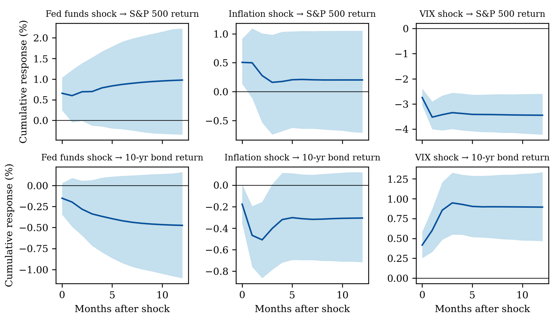
Table 9. Cumulative orthogonalised impulse responses (%), with 95% Monte Carlo bands
Shock → response | Impact (h = 0) | h = 1 | h = 3 | h = 6 | h = 12 |
Fed funds → EQ | 0.66† [0.25, 1.04] | 0.60 [−0.05, 1.22] | 0.70 [−0.13, 1.53] | 0.87 [−0.21, 1.91] | 0.98 [−0.34, 2.23] |
Inflation → EQ | 0.51† [0.14, 0.91] | 0.50 [−0.11, 1.09] | 0.16 [−0.74, 0.98] | 0.21 [−0.64, 1.05] | 0.20 [−0.71, 1.05] |
GDP growth → EQ | 0.34 [−0.03, 0.73] | 0.53 [−0.11, 1.11] | 0.44 [−0.37, 1.16] | 0.41 [−0.66, 1.41] | 0.42 [−1.01, 1.73] |
VIX → EQ | −2.74† [−3.05, −2.38] | −3.52† [−4.00, −2.90] | −3.34† [−3.99, −2.55] | −3.42† [−4.11, −2.63] | −3.45† [−4.21, −2.59] |
Unemployment → EQ | 0.13 [−0.28, 0.52] | 0.37 [−0.25, 0.93] | 0.31 [−0.41, 0.95] | 0.36 [−0.35, 1.02] | 0.38 [−0.36, 1.08] |
Fed funds → BOND | −0.15 [−0.34, 0.03] | −0.20 [−0.49, 0.09] | −0.34 [−0.72, 0.07] | −0.42 [−0.92, 0.12] | −0.47 [−1.10, 0.16] |
Inflation → BOND | −0.18 [−0.35, 0.01] | −0.47† [−0.76, −0.19] | −0.40 [−0.79, 0.01] | −0.31 [−0.70, 0.10] | −0.31 [−0.71, 0.12] |
VIX → BOND | 0.42† [0.25, 0.58] | 0.60† [0.33, 0.87] | 0.95† [0.55, 1.33] | 0.90† [0.51, 1.29] | 0.89† [0.47, 1.34] |
Unemployment → BOND | 0.06 [−0.13, 0.24] | −0.09 [−0.39, 0.19] | −0.17 [−0.57, 0.21] | −0.18 [−0.57, 0.19] | −0.21 [−0.62, 0.18] |
Fed funds → ΔVIX | −3.88† [−5.61, −2.07] | −3.80† [−6.14, −1.35] | −3.23† [−5.84, −0.42] | −2.87 [−6.10, 0.58] | −2.38 [−6.11, 1.45] |
GDP growth → ΔVIX | −1.75† [−3.49, −0.01] | −1.60 [−3.98, 0.95] | −0.64 [−3.05, 2.25] | −0.04 [−3.17, 3.70] | 0.59 [−3.42, 4.77] |
Source: Author’s Compilation Note: Cholesky ordering GDPG, ΔUN, ΔINF, ΔFFR, ΔVIX, BOND, EQ. h = months after the shock. † = 95% band excludes zero. Bands from 1,000 Monte Carlo replications. | |||||
The variance decomposition confirms the ranking. At a twelve-month horizon, VIX shocks account for 55.5% of the forecast-error variance of equity returns, whereas the federal funds rate, inflation, GDP and unemployment together account for 6.9%. For bonds, VIX shocks account for 8.1% and inflation shocks for 3.9%; most bond variance is due to the bond’s own shock. The results are robust to lag length and ordering: with four lags, the twelve-month equity response to a VIX shock is −3.16%, and when the VIX is ordered first it is −3.63%. The positive equity response to rate shocks, however, shrinks to 0.10% when the VIX is ordered before the policy rate, consistent with the view that this response reflects the Fed’s reaction to market conditions rather than a structural effect of policy.
Long-run relations: Johansen cointegration tests
Table 10 reports the Johansen tests for each system separately, with the full sequence of rank tests. For the equity system neither the trace nor the maximum-eigenvalue statistic rejects the null of no cointegration (r = 0: trace 36.45 against a critical value of 47.85). There is therefore no evidence of a stable long-run equilibrium between the level of the S&P 500 and the levels of output, prices and the policy rate over 1994–2023, in contrast to evidence reported for some emerging markets (Keswani et al., 2024). The large swings in valuation ratios during the sample, including the dot-com boom and the post-2009 expansion, make such an equilibrium hard to detect. For the bond system both tests indicate one cointegrating vector (r = 0 rejected, r ≤ 1 not rejected). Normalised on the 10-year yield, the vector implies GS10 = 0.385 FFR − 4.96 ln CPI + constant. The long rate therefore moves with the policy rate in the long run, consistent with the expectations component of the term structure, while the negative price-level term captures the secular decline of long-term yields over the sample. We treat this vector as a statistical description of shared trends rather than a structural relation.
Table 10. Johansen cointegration tests
System | H₀: rank ≤ r | Trace | 5% c.v. | Max-eigenvalue | 5% c.v. |
Equity: ln S&P 500, ln GDP, ln CPI, FFR (lags in differences: 3) | r = 0 | 36.45 | 47.85 | 19.63 | 27.59 |
r = 1 | 16.82 | 29.80 | 11.35 | 21.13 | |
r = 2 | 5.47 | 15.49 | 5.24 | 14.26 | |
r = 3 | 0.24 | 3.84 | 0.24 | 3.84 | |
Bond: GS10, FFR, ln CPI (lags in differences: 1) | r = 0 | 34.26** | 29.80 | 30.08** | 21.13 |
r = 1 | 4.18 | 15.49 | 3.77 | 14.26 | |
r = 2 | 0.42 | 3.84 | 0.42 | 3.84 | |
Source: Author’s Compilation Note: Unrestricted constant, no trend; lag order selected by BIC in the levels VAR. ** = rejection at 5%. | |||||
Regime dependence
Table 11 tests H6 with regime interactions. For equities the interactions are jointly significant in all three regimes (recession: χ²(5) = 37.60; high VIX: 32.69; high inflation: 23.42; all p < 0.001). The sensitivity to the VIX rises from −0.139 in expansions to −0.222 in recessions and from −0.110 to −0.201 in high-volatility months, so equity sensitivity to VIX changes is roughly 60–80% larger in stressed markets. The equity response to inflation is much larger in recessions (2.753 against 0.431). In expansions, rising unemployment is associated with lower equity returns (−1.788, p <0.001); this differs from the finding of Boyd et al. (2005) for an earlier period.
Table 11. Regime-dependent coefficients from interaction models
Regressor | Expansion | Recession | Low VIX | High VIX | Inflation ≤ 3% | Inflation > 3% |
EQ: ΔFFR | −1.995 | −2.679 | −1.046 | −0.294 | 0.357 | 1.051 |
EQ: ΔINF | 0.431 | 2.753***‡ | 0.466* | 1.544** | 1.303** | 0.778* |
EQ: GDPG | 0.073 | −0.212 | 0.109 | −0.030 | 0.043 | 0.185 |
EQ: ΔVIX | −0.139*** | −0.222***‡ | −0.110*** | −0.201***‡ | −0.146*** | −0.195***‡ |
EQ: ΔUN | −1.788*** | −0.153‡ | −1.691*** | −0.329‡ | −0.237 | −4.438**‡ |
EQ: Wald χ²(5), interactions = 0 | 37.60 [<0.001] | 32.69 [<0.001] | 23.42 [<0.001] | |||
EQ: months in regime | 332 | 28 | 270 | 90 | 263 | 97 |
BOND: ΔFFR | −1.368** | 2.912***‡ | 0.070 | −1.802* | −1.298 | −0.833 |
BOND: ΔINF | −0.624*** | −3.079***‡ | −0.832*** | −0.463 | −1.190*** | 0.297‡ |
BOND: GDPG | −0.016 | 0.795***‡ | 0.041 | 0.049 | 0.019 | −0.069 |
BOND: ΔVIX | 0.015* | 0.020 | −0.002 | 0.030**‡ | 0.021*** | −0.000 |
BOND: ΔUN | 0.445 | 0.604*** | 0.601 | 0.130 | 0.092 | −0.702 |
BOND: Wald χ²(5), interactions = 0 | 45.77 [<0.001] | 8.13 [0.149] | 12.45 [0.029] | |||
BOND: months in regime | 332 | 28 | 270 | 90 | 263 | 97 |
Source: Author’s Compilation Note: Each pair of columns comes from one regression that interacts all regressors with the regime dummy. Entries are the coefficient in each regime (base coefficient, and base plus interaction); significance from HAC (5-lag) tests. ‡ = the difference between regimes is significant at 5%. p-values of the Wald test in brackets. *, ** and *** denote 10%, 5% and 1%. | ||||||
For bonds, the recession interactions are jointly significant (χ²(5) = 45.77, p <0.001): the inflation coefficient falls from −0.624 in expansions to −3.079 in recessions, while the policy-rate coefficient changes sign. Because only 28 recession months are available, these recession estimates are imprecise and should be interpreted with caution. The high-inflation interactions are also significant (p = 0.029). Surprisingly, inflation changes lower bond returns significantly when inflation is at or below 3% (−1.190, p <0.001) but not when it is above 3% (0.297, p = 0.447). One possible explanation is that in high-inflation months (about a third of which fall in 2021–2023), bond prices were driven mainly by expectations about the policy-rate path rather than by monthly inflation news. The high-VIX interactions for bonds are not jointly significant (p = 0.149).
Table 12 shows that the stock–bond correlation is itself regime dependent. It is −0.300 in high-volatility months and 0.067 otherwise (p = 0.002), the flight-to-quality effect documented by Connolly et al. (2005). It is −0.348 when GDP growth is below 2% but close to zero otherwise (p = 0.002). When inflation exceeds 3%, it rises to about zero (0.045 against −0.254; p = 0.011), which is consistent with bonds losing their hedging value when inflation risk dominates (Baele et al., 2010; Campbell et al., 2017). By sub-period, the correlation was −0.068 in 1994–2007, −0.333 in 2008–2019 and 0.015 in 2020–2023. The recession difference is not significant, again because of the small number of recession months.
Table 12. Cross-asset correlations by regime
Regime split | Months (regime / other) | Stock–bond corr., regime | Stock–bond corr., other | Fisher z | p-value | Stock–VIX corr., regime / other |
Recession vs expansion | 28 / 332 | −0.329 | −0.091 | −1.20 | 0.229 | −0.88 / −0.67 |
High vs low VIX | 90 / 270 | −0.300 | 0.067 | −3.05 | 0.002 | −0.81 / −0.60 |
Inflation >3% vs ≤3% | 97 / 263 | 0.045 | −0.254 | 2.53 | 0.011 | −0.81 / −0.69 |
GDP growth <2% vs ≥2% | 108 / 252 | −0.348 | −0.006 | −3.07 | 0.002 | −0.81 / −0.65 |
1994–2007 | 168 | −0.068 | — | — | — | −0.66 |
2008–2019 | 144 | −0.333 | — | — | — | −0.72 |
2020–2023 | 48 | 0.015 | — | — | — | −0.84 |
Source: Author’s Compilation Note: Pearson correlations of monthly EQ with BOND and with ΔVIX. Fisher z-test of equal stock–bond correlations across the two groups. | ||||||
Finally, the two-state Markov-switching model (Table 13, Figure 3) identifies regimes without imposing dates. The first regime is calm: its residual variance is 2.69, the mean return is 1.40% per month and the regime lasts 18.5 months on average. The second is turbulent: its variance is 9.44, the mean return is −0.31% (not significant) and it lasts 10.1 months. The turbulent regime covers 32.8% of months and also includes part of the 1999 boom, but otherwise tracks known episodes of market stress: the 1997–1998 Asian and LTCM crises, the 2000–2003 bear market, the 2008–2009 crisis, the 2010–2011 euro-area crisis, shorter spells in 2015–2016 and late 2018, the COVID-19 shock of 2020 and the 2022 tightening cycle. In the calm regime the federal funds rate coefficient is negative and significant (−3.881, p = 0.001), which supports H1; in the turbulent regime it is positive and insignificant (1.494, p = 0.175). The VIX coefficient doubles from −0.105 to −0.210. These results reconcile the full-sample findings: higher policy rates are associated with lower equity returns when markets are calm, but in turbulent periods the Fed’s reaction to falling prices dominates, and the full-sample coefficient averages the two. Table 14 shows the decision of each hypothesis used in our study.
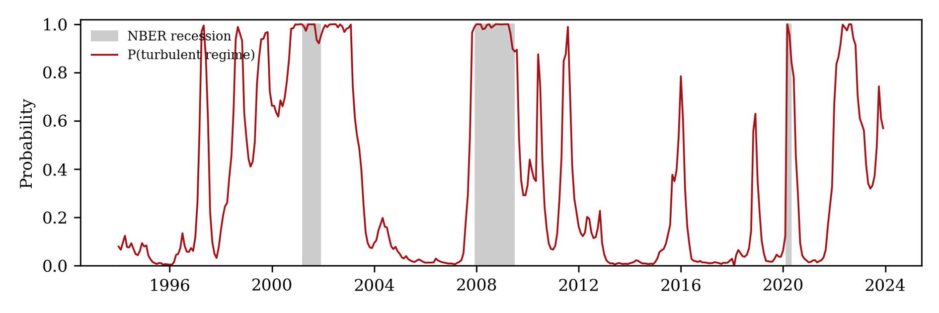
Table 13. Two-state Markov-switching regression for equity returns
Parameter | Regime 1 (calm) | Regime 2 (turbulent) |
Constant | 1.401*** | −0.314 |
ΔFFR | −3.881*** | 1.494 |
ΔVIX | −0.105*** | −0.210*** |
Residual variance | 2.692 | 9.445 |
Probability of staying in regime | 0.946 | 0.901 |
Expected duration (months) | 18.5 | 10.1 |
Log-likelihood | −803.09 | |
Source: Author’s Compilation Note: Dependent variable EQ (% per month); coefficients per unit change in the regressor; switching intercept, slopes and variance; N = 360. *, ** and *** denote significance at 10%, 5% and 1%. | ||
Table 14. Decision on each hypothesis
Hypothesis | Decision | Main evidence |
H1: ΔFFR → lower EQ and BOND | Partly supported | Bonds: −1.144** (full sample). Equities: negative in 1994–2007 (−2.466*) and in the calm Markov regime (−3.881***); not in the full sample. |
H2: ΔINF → lower BOND | Supported | −0.778***; Granger p = 0.037; lagged effect −0.799**. |
H3: GDPG → higher EQ | Partly supported | Significant in 1994–2007 (0.535**); not significant in the full sample. |
H4a: ΔVIX → lower EQ | Supported | −0.162***; VIX explains 56% of EQ forecast variance. |
H4b: macro → ΔVIX | Largely not supported | No macro variable Granger-causes the VIX; contemporaneous links vanish without 2020; the VIX falls after policy-rate shocks in the VAR, most likely reflecting the Fed’s reaction to markets. |
H5: lagged ΔUN → returns | Not supported | Joint lag test significant for EQ only because of 2020 (p = 0.683 without it). |
H6: regime dependence | Supported | Wald tests of interactions (p < 0.001 for EQ), Fisher z-tests on stock–bond correlation, Markov-switching slopes. |
Source: Author’s Compilation | ||
Discussion
The bond results are the most robust part of the evidence. The negative association between inflation changes and Treasury returns holds in the full sample, after 2008, without the COVID-19 months and in a predictive specification, and it is supported by the Granger test. It is not significant in 1994–2007, when inflation was low and stable, and the impulse response is significant only in the first month. Its size is economically relevant: a one-standard-deviation inflation change (0.41 pp) is associated with a bond-return change of about 0.32%, close to the average monthly bond return. This matches the long-standing finding that inflation news is the main macroeconomic driver of nominal bond prices (Ang & Piazzesi, 2003; Campbell & Ammer, 1993; Flannery & Protopapadakis, 2002). The policy-rate effect on bonds is also negative, but it is less precisely estimated in the VAR, as expected when monthly rate changes are largely anticipated.
For equities, macroeconomic variables explain little of monthly return variation once option-implied volatility is taken into account. This agrees with Flannery and Protopapadakis (2002), who find that few macroeconomic series are priced, and with evidence that the variance risk premium embedded in the VIX captures time-varying risk aversion (Bekaert & Hoerova, 2014). The absence of a negative full-sample relation between policy-rate changes and equity returns should not be read as evidence that monetary policy does not matter for stocks. The event-study literature measures exogenous surprises within minutes of an announcement (Bernanke & Kuttner, 2005; Gertler & Karadi, 2015), while monthly changes combine surprises with the Fed’s systematic reaction to markets. Our sub-sample and Markov-switching estimates are consistent with this: the expected negative effect appears before 2008 and in calm regimes, when the policy rate was not responding to market stress, and it disappears when the Fed eased aggressively during crises and when the policy rate was at the zero lower bound. The positive relation between inflation changes and equity returns after 2008 is in line with the change in the sign of the inflation–stock relation reported by Boons et al. (2020) and with the shift of bonds from inflation bets to deflation hedges (Campbell et al., 2017).
The regime results are the main new evidence. Equity sensitivity to volatility shocks is substantially larger in recessions and in high-volatility months, the stock–bond correlation is negative in stress and close to zero when inflation is high, and a data-driven Markov-switching model separates a calm regime, in which interest rates behave as asset-pricing theory predicts, from a turbulent regime in which they do not. These findings support the regime-switching view of asset returns (Ang & Bekaert, 2002; Guidolin & Timmermann, 2007) and the evidence that macroeconomic uncertainty has regime-dependent effects on US market volatility (Liu & Garrett, 2023). They also show why full-sample linear estimates, including those in our Table 5, can be misleading when regimes with opposite signs are pooled.
Three qualifications apply. First, all coefficients are conditional associations, and the Granger tests measure predictive content, so neither establishes causality. Second, the recession estimates rest on 28 months and are imprecise. Third, the lack of cointegration in the equity system does not mean that macroeconomic fundamentals are irrelevant for long-run valuations; it means that no stable linear equilibrium in levels can be identified over this sample.
Practical and Policy Implications
Policymakers. Inflation news is closely and consistently associated with Treasury returns, and a VIX shock is followed by a cumulative equity decline of about 3.4% with no reversal within a year. Central banks assessing the financial-conditions channel should therefore monitor option-implied volatility alongside the policy rate. Because the stock–bond correlation rises to about zero when inflation exceeds about 3%, the stabilising role of Treasuries in private portfolios weakens precisely when inflation is high, which is relevant for financial-stability assessments during tightening cycles.
Investors and portfolio managers. The diversification benefit of nominal bonds is regime dependent: bonds hedge equities in high-volatility and low-growth months but not in high-inflation months. Allocation rules based on a single long-run correlation will overstate the hedge in inflationary periods. Regime indicators such as the VIX level, the inflation rate or the Markov-switching probability can be used to adjust bond–equity weights or to add inflation-protected securities when inflation exceeds 3%.
Risk managers and financial institutions. Stress tests should use regime-specific sensitivities. The equity sensitivity to a volatility shock in recessions is about 1.6 times its expansion value, so applying full-sample betas would understate losses in exactly the scenarios that matter. Duration exposure should be assessed against inflation news, which is the macroeconomic variable most consistently associated with Treasury returns in our data.
Derivatives users. Because macroeconomic variables neither predict monthly changes in the VIX nor explain much of their contemporaneous variation, monthly macroeconomic forecasts are unlikely to add much to option pricing or volatility hedging. Regime indicators and measures of market stress, which are strongly related to equity returns and to the stock–bond correlation in our results, appear more informative for managing volatility exposure.
Conclusion, Limitations and Future Research
This study examined how monetary policy, inflation, real activity, unemployment and volatility relate to US equity, Treasury and index-option markets from 1994 to 2023, using documented public data and a sequence of complementary methods. Inflation increases are consistently associated with lower Treasury returns, and policy-rate increases are also associated with lower returns, although less robustly. Equity returns are dominated by option-implied volatility, and the expected negative association between the policy rate and equity returns appears only in calm market regimes and, weakly, before 2008. Equity sensitivities to macroeconomic variables differ significantly across recessions, high-volatility periods and high-inflation periods, and the stock–bond correlation differs across volatility, growth and inflation regimes.
Each limitation points to a specific extension. (1) Monthly changes in the policy rate are endogenous; future work could use high-frequency policy surprises (Bauer & Swanson, 2023; Jarociński & Karadi, 2020) or external instruments to identify causal effects. (2) The analysis is limited to the US; a cross-country panel would show whether the regime patterns hold where the currency is not a reserve currency. (3) Swap spreads could not be analysed with consistent public data; with licensed data, the same framework could be extended to swaps and futures. (4) Regimes were defined by observable thresholds or by a two-state model; time-varying-parameter VARs, multiple-break tests (Bai & Perron, 1998) and machine-learning methods that capture non-linearities (Gu et al., 2020) could characterise the dynamics more flexibly. (5) Geopolitical and policy uncertainty were not modelled explicitly; published indices (Baker et al., 2016; Caldara & Iacoviello, 2022) could be added as state variables.
Author Contributions
M. Faheem Ullah: Conceptualization, Investigation, Writing – original draft, Writing – review & editing, Validation, Visualization.
Joseph Falzon: Conceptualization, Writing – original draft, Writing – review & editing, Formal analysis, Project administration, Methodology, Software.
Declaration of Competing Interest
The authors declare no conflicts of interest.
Ethics Statement
Not applicable.
Data Availability
Data available on request from the corresponding author.